Generate Local Spectrograms¶

Local spectrograms are computed from downloaded FLAC/WAV audio. You control the FFT window, overlap, frequency range, colour scale, backend, and saved formats.

If you have not downloaded audio yet, start with Download Audio or the complete audio-to-spectrogram walkthrough.

Choose the local workflow¶

Workflow	What it does	Clip-boundary handling
`process_single_file()` / `process_directory()`	Computes a spectrogram from a complete local audio file	Uses only complete STFT windows; it does not add artificial samples beyond the file
`clip_start` / `clip_end` or `--clip-start` / `--clip-end`	Computes a selected interval from local audio	Uses automatic half-window context by default, then removes it
`process_event()`	Computes around a known time in one local audio file	Automatically reads an extra half-window on each side, then removes that context
`--event-time` command-line mode	Command-line form of `process_event()`	Same automatic half-window context and trimming
`create_custom_spectrograms_from_json()`	Downloads ONC audio for timestamped events and computes spectrograms locally	Automatically downloads extra context, computes the STFT, and trims back to the requested interval
`download_requests_from_json()`	Downloads spectrogram products computed by ONC	Processing at product boundaries is controlled by ONC

Use create_custom_spectrograms_from_json() when you want the FFT and plotting settings in the JSON file to control newly computed local spectrograms. Use download_requests_from_json() when you want ONC's existing or server-generated spectrogram products.

Process an audio directory¶

from pathlib import Path

from onc_hydrophone_data.audio import SpectrogramGenerator

audio_dir = Path("data/DEVICE/RUN/audio")
output_dir = audio_dir.parent / "custom_spectrograms"

generator = SpectrogramGenerator(
    win_dur=0.5,
    overlap=0.75,
    freq_lims=(20, 10_000),
    crop_freq_lims=True,
    clim=(-60, 0),
    log_freq=False,
)

results = generator.process_directory(
    audio_dir,
    output_dir,
    save_plot=True,   # PNG
    save_mat=True,    # MATLAB arrays + metadata
    save_npy=False,
    max_workers=4,
)

One successful result contains png_file, mat_file, audio metadata, and processing settings. Batch results omit the large in-memory arrays by default to keep memory use bounded.

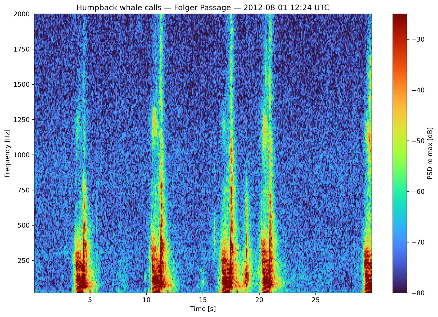
Local spectrogram of ONC humpback whale calls recorded at Folger Passage

The real ONC recording contains repeated humpback calls with acoustic energy that changes over time and frequency.

Choose useful parameters¶

Setting	Start with	Effect
`win_dur`	`0.5` s	Longer windows improve frequency detail; shorter windows improve timing detail
`overlap`	`0.5`–`0.75`	Higher overlap creates more time columns and costs more compute
`freq_lims`	Your band of interest	Controls the plotted frequency range
`crop_freq_lims`	`True` for focused work	Also removes out-of-band rows from MAT/NumPy output, saving disk and memory
`clim`	`(-60, 0)`	Sets contrast in relative dB plots
`log_freq`	`False` initially	Use `True` when several frequency decades must fit on one axis
`backend`	`"auto"`	Uses an available optimized backend and falls back to SciPy when needed

Window length trade-off¶

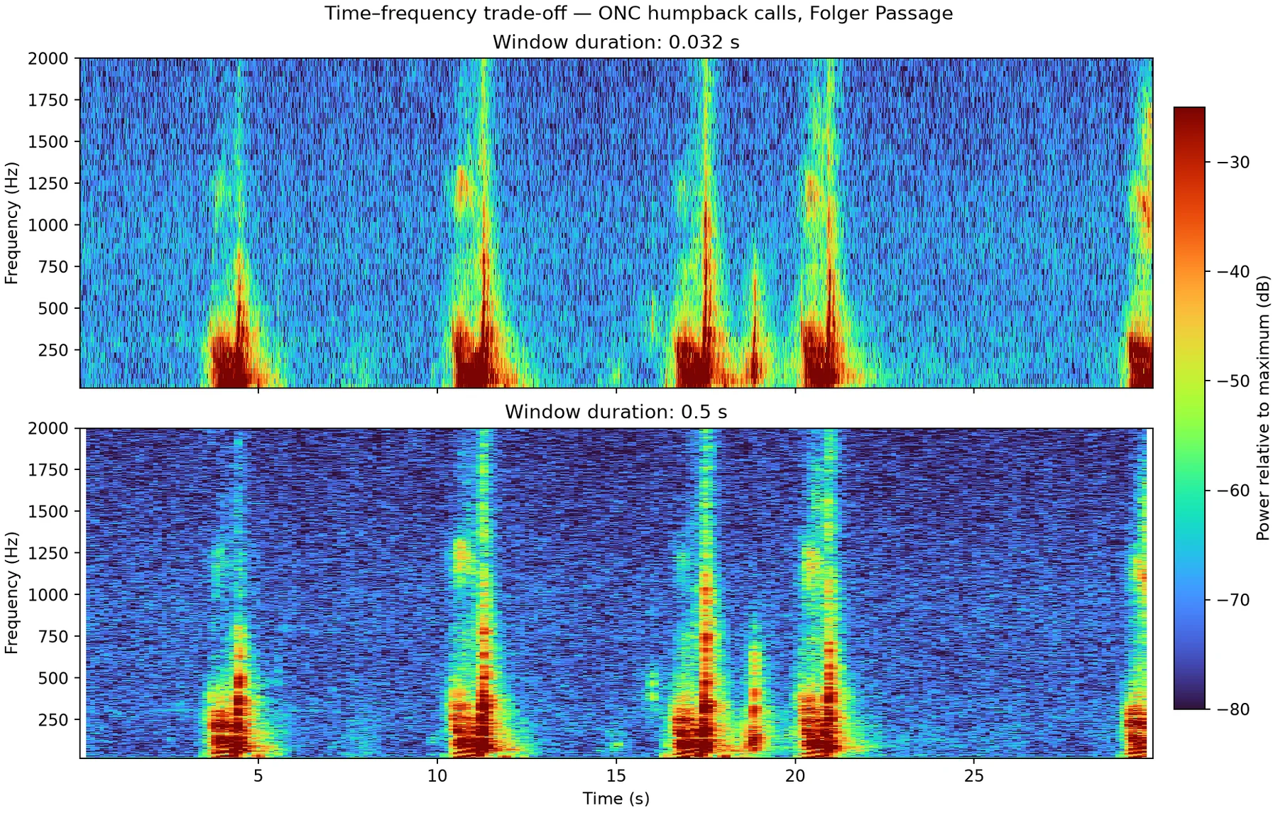
Comparison of short and long spectrogram windows

The short window keeps brief events narrow in time but produces broader frequency bands. The long window sharpens steady tones and sweeps in frequency but spreads short events across time.

Source recording

Both figures are generated by scripts/generate_docs_figures.py from a public ONC recording made by ICLISTENHF1205 at Folger Passage on 2012-08-01 at 12:24 UTC. The script downloads ONC's public audio preview by default, or accepts an ONC audio file with --audio-file. See the ONC source record. The plots use relative power and are not calibrated sound-pressure level.

Process one file¶

result = generator.process_single_file(
    audio_dir / "example.flac",
    output_dir,
    save_plot=True,
    save_mat=True,
    save_npy=True,
)

print(result["png_file"])
print(result["mat_file"])
print(result["npy_file"])

Use the single-file form while tuning parameters, then process the whole directory after the output looks right.

Command-line workflow¶

From a cloned repository checkout:

python scripts/generate_spectrograms.py \
    --input-dir data/DEVICE/RUN/audio \
    --output-dir data/DEVICE/RUN/custom_spectrograms \
    --win-dur 0.5 \
    --overlap 0.75 \
    --freq-min 20 \
    --freq-max 10000 \
    --crop-freq-lims \
    --max-workers 4

Run python scripts/generate_spectrograms.py --help for every option.

Generate around a known signal time¶

Use event mode when a signal occurs at a known offset in an existing audio file. The default retains five seconds before and after the event. It also reads an extra half-window of audio on each side while computing the STFT, then keeps only frames centred inside the requested ten-second interval. This ensures that every retained time bin is calculated from a complete analysis window.

result = generator.process_event(
    audio_dir / "example.flac",
    output_dir,
    event_time_seconds=123.4,
    pad_before_seconds=5,
    pad_after_seconds=5,
    edge_padding_seconds="auto",
    save_plot=True,
    save_mat=True,
)

edge_padding_seconds="auto" is the default and resolves to half the actual STFT window after the audio sample rate and any win_length override are known. The resolved value, event time, target interval, and retained padding are stored in the output metadata.

The same mode is available from the command line:

python scripts/generate_spectrograms.py \
    --input-file audio/example.flac \
    --event-time 123.4 \
    --event-pad-before 5 \
    --event-pad-after 5 \
    --output-dir spectrograms

Generate local event spectrograms from JSON¶

For many labeled events, one workflow can download the needed audio context, clip each event, and generate local spectrograms:

from onc_hydrophone_data.data import HydrophoneDownloader
from onc_hydrophone_data.onc.common import load_config

onc_token, data_dir = load_config()
dl = HydrophoneDownloader(onc_token, data_dir)

results = dl.create_custom_spectrograms_from_json(
    "custom_requests.json",
    clip_pad_seconds="auto",
    save_mat=True,
    save_png=True,
)

{
  "defaults": {
    "deviceCode": "ICLISTENHF6324",
    "pad_seconds": 10
  },
  "generator_defaults": {
    "win_dur": 0.5,
    "overlap": 0.75,
    "freq_lims": [20, 10000],
    "crop_freq_lims": true
  },
  "requests": [
    {
      "timestamp": "2024-04-01T12:30:00Z",
      "label": "example event",
      "generator_options": {
        "log_freq": false
      }
    }
  ]
}

The workflow requests adjacent source files when padding crosses a five-minute boundary. With clip_pad_seconds="auto", it adds half of the configured win_dur on both sides before computing the STFT, removes that context before relative-dB normalization, and returns only time bins centred inside the requested event interval. This prevents incomplete-window artifacts at the requested clip boundaries. If generator_options sets a sample-based win_length that differs from win_dur, set clip_pad_seconds explicitly in seconds so the download context matches that window.

This edge handling applies to spectrograms computed locally by this package. Spectrograms returned by download_requests_from_json() or the other ONC spectrogram download methods are computed by ONC and follow ONC's processing.

Understand the saved values¶

P is the uncalibrated power spectrogram.
PdB_norm is power in dB relative to the maximum value in that file.
F contains frequency-bin centres in hertz.
T contains time-bin centres in seconds.
Metadata records the source audio and FFT/generator settings.

Important

Local outputs are not automatically calibrated sound-pressure levels. If you need ONC calibration or standardized server products, read Choose ONC Server Spectrograms.